I need to note that a lot of this post was inspired by RaviSoji’s PLDA implementation

Preprocessing using PCA

Let us say that we have a training dataset $X \in \mathbb{R}^{N\times F}$ and $y \in \mathbb{R}^N$, where $N$ is the number of examples in the whole dataset, $F$ is the number of features in the dataset, $K$ specifies the number of classes that there are, and $\boldsymbol{m} \in \mathbb{R}^F$ represents the mean vector of the entire dataset $X$.

from mnist import MNIST
from sklearn.decomposition import PCA
import scipy
ds = MNIST("/home/data/MNIST")
ds.gz = True
images, labels = ds.load_training()
X = np.array(images)#.reshape(-1,28,28)
y = np.array(labels)
K = len(np.unique(y))
F = len(X[0])
m = np.mean(X,axis=0)

For a classification problem we will create several subspaces:

• $\mathcal{D}$ represents the space where the data lives in
• $\mathcal{X}$ represents the subspace found via PCA where the data in $\mathcal{D}$ gets transformed to the subspace $\mathcal{X}$. Here, you may consider $\mathcal{X}$ to be the space of the preprocessed state
• $\mathcal{U}$ represents the subspace found via PLDA, where the data will be ultimately transformed to, which is described in detail by Ioffe 2006
• $\mathcal{U}_{model}$ represents the subspace within $\mathcal{U}$ which contains only the dimensions that are relevant to the problem

So, in general, the data will first flow in the following fashion \(\mathcal{D} \leftrightarrow \mathcal{X} \leftrightarrow \mathcal{U} \leftrightarrow \mathcal{U}_{model}\)

First, for a classification problem, we perform a PCA to reduce the dimensionality, and get rid of features that may not be very important. In other words, we will bring the data from $\mathcal{D}$ to $\mathcal{X}$. For this one needs to determine the number of components that one would want to take into account for in its subspace, and set that as the matrix rank. This can be predefined or not. If it is not defined, we compute the covariance matrices for each of the classes (i.e. a between-class covariance matrix and a within-class covariance matrix per class $k$). In other words

For each class

1. Compute the mean vectors $m_k \in \mathbb{R}^F$
2. Compute the covariance matrix $\sigma_k \in \mathbb{R}^{F\times F}$
3. Compute the between-class covariance matrix per class $S_{b,k} \in \mathbb{R}^{F\times F}$ \(S_{b,k} = \frac{n_k}{N}\underbrace{(\boldsymbol{m}_k - \boldsymbol{m})^T}_{\mathbb{R}^{F\times 1}} \underbrace{(\boldsymbol{m}_k - \boldsymbol{m})}_{\mathbb{R}^{1\times F}}\)
4. Compute the within-class covariance matrix per class $S_{w,k} \in \mathbb{R}^{F\times F}$ \(S_{w,k} = \frac{n_k-1}{N} \odot \sigma_{k}\)

Then compute the within-class and between-class covariance matrices, $S_w \in \mathbb{R}^{F\times F}$ and $S_b \in \mathbb{R}^{F\times F}$ respectively. If one was to set \(\boldsymbol{m}_{ks} \in \mathbb{R}^{K\times F}\) as the matrix representing all of the mean vectors, $\boldsymbol{\sigma_{ks} \in \mathbb{R}^{K\times F \times F}}$ the tensor representing all of the class covariances, and $n_{ks}\in \mathbb{R}^K$ a vector representing all of the number of examples in each class, it is possible to vectorize it all as

n_principal_components = None # This might overfit

if n_principal_components:
    matrix_rank = n_principal_components
else:
    m_ks, sigma_ks, n_ks = [],[],[]
    for k in range(K):
        # Get only the data associated with class k
        X_k = X[y==k]
        
        # Compute the mean, number of samples, and class covariance
        m_k = np.mean(X_k,axis=0)
        n_k = len(X_k)
        sigma_k = np.cov(X_k.T)
        
        # Append them all
        m_ks.append(m_k)
        n_ks.append(n_k)
        sigma_ks.append(sigma_k)
    m_ks = np.array(m_ks)
    n_ks = np.array(n_ks)
    sigma_ks = np.array(sigma_ks)
    
    assert m_ks.shape == (K,F)
    assert n_ks.shape == (K,)
    assert sigma_ks.shape == (K,F,F)
    
    S_b =  ((m_ks - m).T * n_ks/N)  @ (m_ks - m)
    S_w = np.sum(sigma_ks * ((n_ks-1)/N).reshape(-1,1,1), axis=0)
    
    matrix_rank = np.linalg.matrix_rank(S_w)

if F != matrix_rank:
    pca = PCA(n_components = matrix_rank)
    pca.fit(X)

Now, there are going to be several transformations:

• $\mathcal{D} \rightarrow \mathcal{X}$

Here, there are two case scenarios. If PCA was defined in order to reduce the dimensions, then the data in $\mathcal{D}$ will be transformed via PCA. Otherwise, you can return the data itself

• $\mathcal{X} \rightarrow \mathcal{D}$

In this case, it is very similar to the converse. If PCA was defined, in order to bring it back to the original data space $\mathcal{D}$, you need to inverse transform the data. Otherwise, just return the data itself

def transform_from_D_to_X(x):
    global pca
    if pca:
        return pca.transform(x)
    else:
        return x

def transform_from_X_to_D(x):
    global pca
    if pca:
        return pca.inverse_transform(x)
    else:
        return x

So, at this point, we convert the training data from $\mathcal{D}$ to the space $\mathcal{X}$, having the data be represented as $X_{pca}$

X_pca = transform_from_D_to_X(X)
print("Shape of X_pca =",X_pca.shape)

# Shape of X_pca = (60000, 712)

Probabilistic Linear Discriminant Analysis

Problem Setup

In the PLDA, we use a Gaussian mixture model, where $\boldsymbol{x}$ represents a sample in the mixture, and $\mathcal{y}$ represents the center of a mixture component. In general, the class-conditional distributions is represented by

where all of the class-conditional distributions share one common covariance [I DON’T KNOW WHY THEY ALL SHARE THE SAME COVARIANCE]

If we recall, the LDA formulation is the result if we were to set $\mu_k$ values to be constrainted to be in a lower dimension, and perform the likelihood maximization with respect to $\mu_k$, $\pi_k$, and $\Phi_w$, where the prior of the class variable $\boldsymbol{y}$ is set to put a probability mass on each of the points

But that won’t be the case in the PLDA formulation. Instead, PLDA sets it so that the prior is not to be within a discrete set of values, but instead, sampled from a Gaussian prior.

Note that this normal distribution $P_{PLDA}(y)$ uses the mean of the full dataset. This formulation makes it such that $\Phi_w$ is positive definite, and $\Phi_b$ is positive semi-definite. Theoretically, it is possible to find a transformation $V$ which can simultaneously diagonalize $\Phi_b$ and $\Phi_w$

We can define $A = V^{-T} = \text{inv}(V^T)$, resulting in

Thus, the PLDA model is defined as:

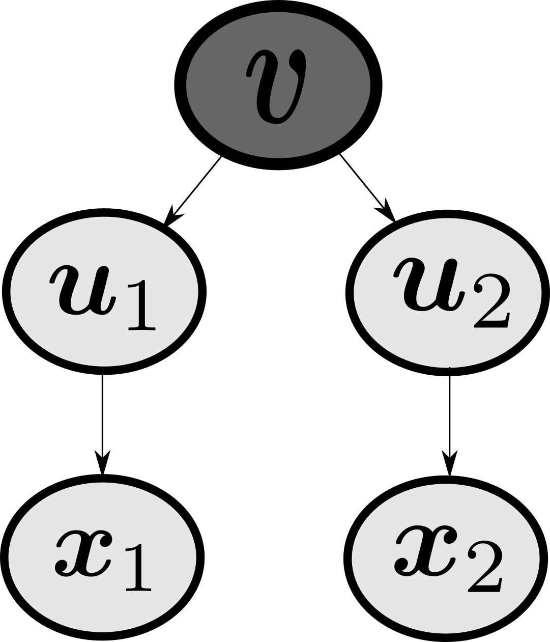
Here, $\boldsymbol{u}$ represents the sample data representation of $\boldsymbol{x}$, but projected in the latent projected space $\mathcal{U}$, and $\boldsymbol{v}$ represents the sample label in the latent projected space. These transformations can be computed via

And from this point on, we determine the optimal $\boldsymbol{m}$, $A$, and $\Psi$ are.

S. Ioffe: “In the training data, the grouping of examples into clusters is given, and we learn the model parameters by maximizing the likelihood. If, instead, the model parameters are fixed, likelihood maximization with respect to the class assignment labels solves a clustering problem”

def transform_from_X_to_U(x):
    global m, A
    return (x-m) @ np.linalg.inv(A)

def transform_from_U_to_X(x):
    global m, A
    return m + (x @ A.T)

But, at this point, we don’t know what the parameters $A$ or $\Psi$ are, so we can’t use these functions yet.

Learning the Model Parameters ($\boldsymbol{m}, \Psi, A$)

The loading matrix $A$ is essentially finding the variances $\Phi_b$ and $\Phi_w$, and all of the parameters can be defined using a maximum likelihood framework. Let us say that $D_k$ represents the dataset which contains only samples from the $k^{th}$ class, and $\boldsymbol{x}_k^i$ represents the $i^{th}$ sample from $D_k$, and it belongs to the $k^{th}$ class. Given $N$ training examples separated into $K$ classes, and assuming that they are all independently drawn from their respective class, the log likelihood is

where the joint probability distribution of a set of $n$ patterns (assuming all these $n$ patterns belong to the same class $k$) is:

By computing the integral, we obtain

where \(\bar{\boldsymbol{x}}_k = \frac{1}{n} \sum_{i=1}^n \boldsymbol{x}^i_k\), and $C$ is a constant that can be ignored

At this point, as a “hack”, it sets the number of examples for each class to be $n$. In other words, every class ends up having exactly $n$ examples to learn from. Now, if one were to maximize the equation $l(\boldsymbol{x}^{1\cdots N})$ with respect to $\boldsymbol{m}$, one would obtain $\boldsymbol{m}^* = \frac{1}{N} \sum_i \boldsymbol{x}^i$. If one substitutes it back, one would get

Now, we need to optimize $l(\boldsymbol{x}^{1\cdots N})$ with respect to $\Phi_b$ and $\Phi_w$ subject to $\Phi_w$ being p.d. and $\Phi_b$ being p.s.d. Without these constraints, we would obtain

Therefore, if $S_w$ and $S_b$ are diagonal, then the covariances $\Phi_w$ and $\Phi_b$ will also be diagonal, and the diagonalization property holds as long as the contraints above are satisfied.

As we have previously stated, we know that

If you fix $\Psi$ and maximize $l(\boldsymbol{x}^{1\cdots N})$ via unconstrained optimization with respect to $A^{-1}$ will make $A^{-1}S_b A^{-T}$ and $A^{-1}S_w A^{-T}$ diagonal. Note that if the scatter matrices $S_w$ and $S_b$ are diagonal, then the covariance matrices $\Phi_w$ and $\Phi_b$ are also diagonal. This will then make the $A^{-T}$ to be the solution of the generalized eigenvector problem involving $S_b$ and $S_w$, where $S_b \boldsymbol{v} = \lambda S_w \boldsymbol{v}$. Then, the projection of the data to the latent space with the LDA projection. [REVIEW]

Then, if you were to optimize $l(\boldsymbol{x}^{1\cdots N})$ with respect to $\Psi$ subject to $\Psi \geq 0$ and $\text{rank}(\Psi) \leq \hat{F}$, then we’ll get the method to optimize the model [REVIEW]

Ioffe 2006: “Our method was derived for the case where each class in the training data is represented by the same number $n$ of examples. This may not be true in practice, in which case, we can resample the data to make the number of examples the same, use EM (as shown in section 5), or use approximations. We took the latter approach, using the closed-form solution in Fig. 2, where $n$ was taken to be the average number of examples per class”

Algorithm: PLDA Optimization

Input: Training $N$ examples from $K$ classes, with $n = N/K$ per class Output: Parameters $\boldsymbol{m}, A, \Psi$, maximizing the likelihood of the PLDA model

1. Compute the covariance matrices $S_b$, and $S_w$
2. Compute the transformation matrix $W$ such that $S_b \boldsymbol{w} = \lambda S_w \boldsymbol{w}$ (i.e. $eig(S_w^{-1}S_b)$)
3. Compute the covariance matrices in the latent space
   • $\Lambda_b = W^T S_b W$
   • $\Lambda_w = W^T S_w W$
4. Determine the following parameters
   • $\boldsymbol{m} = \frac{1}{N} \sum_{i=1}^N \boldsymbol{x}_i$
   • $A = W^{-T} \left( \frac{n}{n-1} \Lambda_w \right)^{1/2}$
   • $\Psi = \max \left( 0, \frac{n-1}{n} (\Lambda_b / \Lambda_w) - \frac{1}{n} \right)$
5. Reduce the dimensionality to $\hat{F}$ by keeping the largest elements of $\Psi$, while setting the rest to zero.
6. In the latent space $\boldsymbol{u} = A^{-1}(\boldsymbol{x}-\boldsymbol{m})$, only the features for non-zero entries are needed for recognition

Note:

Scipy’s eigh(A,B) function in linalg solves the generalized eigenvalue problem for a complex Hermitian or a real symmetric matrix, so that $A\boldsymbol{v} = \lambda B \boldsymbol{v}$. Otherwise, if B is omitted, then it is assumed that $B=I$
Also note that scipy.linalg.eigh != np.linalg.eigh

def compute_Sb_Sw(X,y):
    m = np.mean(X,axis=0)
    _,F = X.shape
    m_ks, sigma_ks, n_ks = [],[],[]
    for k in range(K):
        # Get only the data associated with class k
        X_k = X[y==k]
        
        # Compute the mean, number of samples, and class covariance
        m_k = np.mean(X_k,axis=0)
        n_k = len(X_k)
        sigma_k = np.cov(X_k.T)
        
        # Append them all
        m_ks.append(m_k)
        n_ks.append(n_k)
        sigma_ks.append(sigma_k)
    m_ks = np.array(m_ks)
    n_ks = np.array(n_ks)
    sigma_ks = np.array(sigma_ks)
    
    assert m_ks.shape == (K,F)
    assert n_ks.shape == (K,)
    assert sigma_ks.shape == (K,F,F)
    
    S_b =  ((m_ks - m).T * n_ks/N)  @ (m_ks - m)
    S_w = np.sum(sigma_ks * ((n_ks-1)/N).reshape(-1,1,1), axis=0)
    return S_b, S_w

assert X.shape[0] == y.shape[0]

m = X_pca.mean(axis=0)
n = N/K
S_b, S_w = compute_Sb_Sw(X_pca,y)

# Compute W
eigvals, eigvecs = scipy.linalg.eigh(S_b, S_w)
W = eigvecs

# Compute Lambdas
Lambda_b = W.T @ S_b @ W
Lambda_w = W.T @ S_w @ W

# Compute A
A = np.linalg.inv(W.T) * (n / (n-1) * np.diag(Lambda_w))**0.5
print(A.shape)
# Compute Psi
diag_Lambda_w = Lambda_w.diagonal()
diag_Lambda_b = Lambda_b.diagonal()

Psi = (n - 1)*(diag_Lambda_b/diag_Lambda_w) - (1/n)
Psi[ Psi <= 0 ] = 0
Psi = np.diag(Psi)

From this point you can transform the data that is in the PCA subspace $\mathcal{X}$ to the $\mathcal{U}$ subspace, having the data be represented as $U$

u = transform_from_X_to_U(X_pca)

Now, again, not every dimension will be relevant in the $\mathcal{U}$ subspace, and that is why we reduce the $\mathcal{U}$ to \(\mathcal{U}_{model}\) , which only contains the relevant dimensions of $\mathcal{U}$. Therefore, in order to go back and forth in between the two subspaces, simply drop them the irrelevant dimensions or add the relevant dimensions to a zero matrix. This new data will be represented as $U_{model}$

def transform_from_U_to_Umodel(x,dims):
    u_model = u[...,dims]
    return u_model 

def transform_from_Umodel_to_U(x,dims,u_dim):
    shape = (*x.shape[:-1], u_dim)
    u = np.zeros(shape)
    u[..., dims] = x
    return u

# Compute the relevant dimensions of Psi
relevant_dims = np.squeeze(np.argwhere(Psi.diagonal() != 0)) # [0]
if relevant_dims.ndim == 0:
    relevant_dims = relevant_dims.reshape(1,)

U_model = transform_from_U_to_Umodel(X_pca,relevant_dims)

Great! Now we we have the data in the $\mathcal{U}_{model}$ space. Now, all that there is left is to understand how to perform inference, and in order to do that, one needs to find the prior parameters for $\boldsymbol{v}$, the posterior parameters, and the posterior predictive parameters. Let’s discuss now how to find the probability parameters.

Inference on the Latent Space

First, if you need some review on Bayesian inference for Gaussian distributions, you may check the other post to understand priors, posteriors, posterior predictives, and marginal probability. For this problem, note that the different dimensions have been decorrelated (i.e. the covariances have been decorrelated), thus the different dimensions could be treated as univariate problems.

We need to determing the prior parameters of $\boldsymbol{v}$, which leads to the probability distribution $P(\boldsymbol{v})$, the posterior parameters, which leads to \(P(\boldsymbol{v} \vert \boldsymbol{u})\) , and the posterior predictive parameters, for \(P(\boldsymbol{u}^p \vert \boldsymbol{u}^g_{1\cdots n})\)

Prior Distribution

The easiest to determine right off the bat are the prior parameters. For the prior parameters, as one may recall in the model formulation

which, in turn, are simple to compute. Here we’ll call $\mu_{prior}$ the prior mean, and $\Sigma_{prior}$ the prior covariance, making

where $D$ represents all of the relevant dimensions, which are all that the variances are not zero. Then from this point, we’ll use the notation setting $\hat{\Psi} = \Psi_{\forall d \in D}$

prior_params = {
    "mean": np.zeros(relevant_dims.shape[0]),
    "cov": np.diag(Psi)[relevant_dims]
}

Now, the more involved ones are the posteriors parameters.

One advantage that PLDA has is that it allows one to make inferences about classes not present during training. Let us consider the following case of classification first. We are given a set of data to learn from, which Ioffe refers to as a “gallery”. This set ${ \boldsymbol{x}^1, \cdots,\boldsymbol{x}^k, \cdots, \boldsymbol{x}^K }$ contains $K$ examples, with one example from each of the $K$ classes. We are also given a probe example $\boldsymbol{x}^p$, and assume that it belongs to one of the $K$ classes. If we are to determine to which class it belongs, maximizing the likelihood will do the job. This can be more easily accomplised in the lated space by performing the trnasformation $\boldsymbol{u} = A^{-1}(\boldsymbol{x} - \boldsymbol{m})$, since it will decorrelate the data. For this example, $\boldsymbol{x}^p$ will be transformed to $\boldsymbol{u}^p$.

Next we will see how to compute the posterior distribution and the posterior predictive distribution. We will, however look at two different cases. We will first look in the case where we have a single training example per class (in deep learning, known as $k$-way-one-shot learning), and then we’ll look at the case where we see multiple examples per class (also known as $k$-way-few-shot learning).

Case: Single Training Example per Class

Posterior Distribution

Let us consider an example $\boldsymbol{u}^g$ from the training set (i.e. gallery), where, again, it belongs to some class between $1 \cdots K$ The probability that the probe $\boldsymbol{u}^p$ belongs to the same class as $\boldsymbol{u}^g$ is defined by the probability $P(\boldsymbol{u}^p | \boldsymbol{u}^g)$.

So, the posterior probability will provide a way to perform inference on the class variable $\boldsymbol{v}$ (i.e. the transformed version of $\boldsymbol{y}$). As we may remember, the parameters for a posterior Gaussian are

Now, since we only have a single sample $\bar{x} = \boldsymbol{u}$. Additionally, we know that the mean for the prior $\mu^{prior}$ is all zeros (since the data has been centralized), then

Additionally, since we would be looking at a single class at this point and the covariances have been diagonalized, the within-class covariance is an identity matrix, making the $(\sigma^{prior})^2 = 1$. Therefore the parameters turn into

And, once again, since we are dealing with a single sample, $N=1$

The posterior for a single training example can then be defined as

Now, if we see how this flows, the class variable $\boldsymbol{v}$ will be used to determine $\boldsymbol{u}$ examples, which are then used to determine the data $\boldsymbol{x}$.

Posterior Predictive Distribution

from graphviz import Digraph
dot = Digraph()
dot.node('v',"v")
dot.node('1',"u1")
dot.node('2',"u2")
dot.node("a","x1")
dot.node("b","x2")
dot.edges(['v1',"v2","1a","2b"])
dot

From probabilistic graphical models, if we observe $\boldsymbol{v}$ (i.e. $\boldsymbol{v}$ is given), then $\boldsymbol{u}^p$ and $\boldsymbol{u}^g$ are conditionally independent. We also know that the posterior predictive probability is

And since the within class variance has been diagonalized to an identity matrix ($\sigma^2 = 1$), we’ll obtain

In order to classify $\boldsymbol{u}^p$, then we compute $P(\boldsymbol{u}^p \vert \boldsymbol{u}^g) \forall g \in {1,\cdots,M }$, and pick the maximum.

Ioffe 2006: “With PLDA, we were able to combine the knowledge about the general structure of the data, obtained during training, and the examples of new classes, yielding a principled way to perform classification”

Now that we’ve seen the single example case, let’s expand this to the multiple example case.

Case: Multiple Training Examples Per Class

Posterior Distribution

We can improve the recognition performance by using more examples. Let us say that we have $n_k$ examples from class $k$, making

These examples are all independent examples $\boldsymbol{u}_{1\cdots n}^g$. Just as before, we know that, here, we are looking at a single class $k$. We have previously diagonalized all of the covariance matrices, making all of the dimensions (i.e. features) decorrelated, thus they can be worked on individually as if they were univariate features. This also means that the within-class covariance is an identity matrix, making $\sigma^2 = 1$. As we may remember, the parameters for a posterior Gaussian are

Again, since our model estimates that the prior mean $\mu^{prior}$ is all zeros, then

Since we’re looking at the class $k$, then $N=n_k$ and $\bar{x} = \bar{\boldsymbol{u}}_k$. Thus the posterior for multiple samples is

Therefore, in order to compute the posterior parameters, where $\mu_k^{post}$ and $\Sigma_k^{post}$ are the mean posterior and the covariance posterior for each class $k$, we have

where we can recall that $\Sigma^{prior} = \hat{\Psi}$, and $\bar{\boldsymbol{u}}_k = \frac{1}{n_k}(\boldsymbol{u}_k^1 + \cdots + \boldsymbol{u}_k^{n_k})$

posterior_params = {}
for k in np.unique(y):
    u_model_k = u_model[y==k]
    n_k = len(u_model_k)
    cov = prior_params["cov"] / (1 + n_k * prior_params["cov"])
    mean = np.sum(u_model_k, axis=0) * cov
    posterior_params[k] = {"mean": mean, "cov":cov}

Posterior Predictive Distribution

As per page 535 by Ioffe 2006, if one sets multiple examples of a class to a single model, assuming we have $n_k$ independent examples \(\{ \boldsymbol{u}_k^i \}_{i=1}^{n_k}\), then the probability of obtaining a sample $\boldsymbol{u}^p$, given the set above, can be obtained from the posterior predictive

Once again, since the within-class covariance has been diagonalized to an identity matrix, then $\sigma^2 = 1$

where $\bar{\boldsymbol{u}}_k = \frac{1}{n_k}(\boldsymbol{u}_k^1 + \cdots + \boldsymbol{u}_k^{n_k})$

This means that, you may compute the predictive parameters as copying the posterior parameters ($\mu_k^{postpred}$, $\Sigma_k^{postpred}$), and adding an identity matrix to the covariance

post_pred_params = posterior_params.copy()
for k,params in post_pred_params.items():
    params["cov"] += 1

Summary and Inference

Great! This is all that we need to precompute before performing any inference! At this point, you have determined all of the parameters which describe you data. As a review, in order to prepare this algorithm, we have received a training dataset $X$ and its corresponding labels $y$. Then, we have decided on a certain number of components to be used for a PCA. This PCA will bring the data from the space $\mathcal{D}$ to the space $\mathcal{X}$, obtaining the data $X_{pca}$. Then we found the parameters $\boldsymbol{m}$, $A$, and $\hat{\Psi}$, which optimize the PLDA formulation. These would then allow us to bring the data from the $\mathcal{X}$ subspace to the $\mathcal{U}$ latent space, obtaining the data $U$. Then, we reduced the dimensions of $U$ by discarding any dimensions which had a zero variance in $\hat{\Psi}$, yielding the data $U_{model}$. Finally, using these same parameters, we obtain the prior parameters ($\mu^{prior}$ and $\Sigma^{prior}$), the posterior parameters ($\mu^{post}_k$ and $\Sigma^{post}_k$), and the posterior predictive parameters ($\mu^{postpred}_k$ and $\Sigma^{postpred}_k$)

Now, we’re ready to do the inference on the latent space

We have previously established that we have the classes (i.e. categories) $1,\cdots, K$. What we will do is to iterate through each of the possible classes, and compute its posterior probabilities by using the parameters computed for the posterior predictive probabilities and creating a Gaussian distribution. Finally, we can obtain the probability on that Gaussian at each of those locations. We can also use the log probability for each of the samples on each of the classes

from scipy.stats import multivariate_normal as gaussian
log_prob_post = []
for k, param in post_pred_params.items():
    mean,cov = param["mean"], param["cov"]
    log_probs_k = gaussian(mean,np.diag(cov)).logpdf(U_model)
    log_prob_post.append(log_probs_k)
log_prob_post = np.array(log_prob_post).T

Here, you may choose to normalize the probabilities

normalize = False
if normalize:
    logsumexp = np.log(np.sum(np.exp(log_prob_post),axis=-1))
    log_probs = log_prob_post - logsumexp[..., None]
else:
    log_probs = log_prob_post

categories = np.array([k for k in post_pred_params.keys()])
predictions = categories[np.argmax(log_probs,axis=-1)]

N = len(X)
shape = [3,2]
inds = np.random.choice(N,np.prod(shape))

plt.figure(dpi=200)
fig, ax = plt.subplots(*shape)
count = 0
for i in np.arange(shape[0]):
    for j in np.arange(shape[1]):
        ax[i,j].imshow(X[count].reshape(28,28))
        title = "True: {} | Pred: {}".format(y[count],predictions[count])
        ax[i,j].set_title(title)
        count+= 1

If you wanted to extract the LDA features, you could simply use the transformation functions to convert the data from some space to another space.

So this is the case when we have a classification problem where the probes are assumed to belong to one of the trained classes. Now, let us look at the case where the probes belong to classes not yet seen.

Hypothesis Testing

Here, we try to determine whether two samples belong to the same class or not. For that, we can compute the following likelihoods

As a generalized formulation where there are multiple examples, the likelihood ratio is

where

For the priors $\pi_{\text{same}}$ and $\pi_{\text{diff}}$, the probability that all of the examples are in the same class is

If $R > \pi_{\text{diff}} / \pi_{\text{same}}$, the two groups of examples belong to the same class; otherwise they do not.

The between-class feature variances $\psi_t$ indicate how discriminative the features are. For example, if $\psi=0$, then it is a completely non-discriminative feature.

Therefore, we can compute the marginal likelihoods for each of those possibilities:

• Marginal probability of them being from same class, i.e. $P(\boldsymbol{u}_p^{1\cdots m},\boldsymbol{u}_g^{1\cdots n})$

  Note that, for the marginal probability that they are from the same class, we will are treating it as a single marginal probability \(P(\boldsymbol{u}_p^{1\cdots m},\boldsymbol{u}_g^{1\cdots n}) =P(\underbrace{\boldsymbol{u}_p^1, \cdots, \boldsymbol{u}_p^m}_{\boldsymbol{u}_p^{1\cdots m}},\underbrace{\boldsymbol{u}_g^1, \cdots, \boldsymbol{u}_g^n}_{\boldsymbol{u}_g^{1\cdots n}})\)

• Marginal probability of them being from different classes, i.e. $P(\boldsymbol{u}_p^{1\cdots m}) \cdot P(\boldsymbol{u}_g^{1\cdots n})$

Based on the post about Bayesian inference on Gaussian distributions, we saw that in order to obtain the marginal likelihood on a dataset $\boldsymbol{X}$ is

where $N$ represents the number of examples in $\boldsymbol{X}$, $\sigma^2$ represents the within-class variance, $\bar{x}$ is the mean of the $\boldsymbol{X}$ over all of the $N$ samples, and the $\boldsymbol{x}^i$ represents the $i^{th}$ example in $\boldsymbol{X}$. Now, rewriting this for our example, let us first write this for a single class $k$, considering it to be univariate (remember, we have decorrelated all of the dimensions/features, thus each feature behaves as if it was its on univariate feature)

where, $\sigma_{0,k}^2$ represents the prior variance for the $k^{th}$ class, $\mu_{0,k}$ represents the prior mean for the $k^{th}$ class, and $\sigma_k^2$ represents the within-class variance for the $k^{th}$ class. Do remember, however that we have set the prior means $\mu_{0,k}=0$ for all classes. Therefore

We have also diagonalized our covariance matrices so that the within-class covariance would be the identity matrix. Therefore $\sigma_k^2 = 1$, yielding

But, if we are to have multivariate examples, with $\hat{F}$ features, then we rewrite the formulation above to multiply over the feature dimension $f$

By taking the natural logarithm of it, we can more easily deal with infinitesimal probabilities, and it helps us make multiplications into additions

Since $\sigma_0^2$ represents the prior variance, if we are given a dataset $U_{model}$ with size $n=\vert U_{model}\vert$, we can write the probability of all of those samples occurring as

def marginal_logprob(U):
    n = U.shape[0]
    S_prior = prior_params["cov"]
    log_C = -0.5 * np.log(2*np.pi) - 0.5 * np.log(n*S_prior + 1)
    E1 = 0.5*(n**2 * S_prior * np.mean(U,axis=0)**2)/(n*S_prior + 1)
    E2 = - 0.5 * np.sum(U**2, axis=0)
    logP_t = log_C + E1 + E2 
    logP = np.sum(logP_t, axis=-1)
    return logP

This way, if we were to receive two sets of data

We can set a set by concatenating both of them \(\boldsymbol{u}_{pg} \in \mathbb{R}^{(m+n) \times \hat{F}}\)

And then we can pass them through the computation above

Finally, instead of the ratio, we compute the log of the ratio

In such case, since we are dealing with log ratios, negative values mean that the model believes the two datapoints are from different categories, where as positive values indicate that the model believes that the two data points are from the same category.

logprob_p = marginal_logprob(u_p)
logprob_g = marginal_logprob(u_g)
logprob_pg = marginal_logprob(np.concatenate([u_p,u_g]))
log_Ratio = logprob_pg - (logprob_p + logprob_g)

if log_Ratio > 0:
    print("Belong to the same class")
else:
    print("Belong to different classes")